The Inner Product

The Inner Product, December 2001
Jonathan Blow (jon@number-none.com)
Last updated 13 January 2004

Mipmapping, Part 1

Related articles:

Mipmapping, Part 2 (January 2002)

Welcome to the first installment of The Inner Product, the successor to the column Graphic Content. Graphic Content was first written by Brian Hook in 1997, and the torch was carried by Jeff Lander from 1998 through to the present day.

The new name indicates a change in theme; graphics are important, but we don't want to neglect other areas. How often do you see games ruined by bad AI or faulty network code?

As with Graphic Content, each Inner Product article will be highly technical in nature and come with full source code. My goal is to make this column as useful as possible to experienced and expert game developers. My content guideline is this: if it wouldn't have been new and useful information to me 2 months ago, then I won't write it.

The "inner product", also known as the "dot product", is a mathematical operation on vectors. It's one of the simplest and most useful pieces of 3D math; I chose the name to underscore the importance of mathematics in building game engines. Additionally, the phrase "the inner product" refers to the game engine itself. The people who play your game see a lot of obvious things created by texture artists, 3D modelers, and level designers. But the inner part of the product, the engine, makes it possible for all that art stuff to come together and represent a coherent game world. As such, the engine is all-important.

Though eventually we will cover subjects besides graphics, we're going to start by looking at the process of mipmapping. Our goal is to achieve a sharper display of the entire scene, and perhaps to improve color fidelity too.

What is mipmapping all about?

When mipmapping, we build scaled-down versions of our texture maps; when rendering portions of the scene where low texture detail is needed, we use the smaller textures. Mipmapping can save memory and rendering time, but the motivating idea behind the technique's initial formulation was to increase the quality of the scene by reducing aliasing. Aliasing happens because we're coloring each pixel based on the surface that, when projected to the view plane, contains the pixel center. Small visual details can fit between pixel centers, so that as the viewpoint moves around, they appear and disappear. This causes the graininess that makes Playstation 2 games look icky.

Fortunately for us, a lot of smart people have been thinking about aliasing for a long time; all we have to do is stand on their shoulders.

Way back in 1805, Karl Friedrich Gauss invented the Fast Fourier Transform, a way of decomposing any sampled function into a group of sine waves. The Fourier Transform is more than a mystic voodoo recipe for number crunching; it often presents us with a nice framework for thinking about problems. When manipulating an image, sometimes it's easier to visualize an operator's effect on simple sine waves than on arbitrary shapes.

So how does the Fourier Transform help us here? To eliminate aliasing, we need to throw away all the sine waves with narrow wavelengths -- which represent the only things that can fit between pixels -- and keep the waves with broad peaks. Such a task is performed by a digital filter. For a detailed introduction to filtering and other signal processing tasks, see the books by Steiglitz and Hamming listed in the Further Reading section.

Once we understand that generating mipmaps is just the task of building smaller textures while eliminating aliasing, we can draw on the vast signal processing knowledge built up by those who came before us. So much work has been done already that, once we have the basic concepts, our code almost writes itself.

The Usual Approach to Mipmapping

Historically, game programmers don't think very hard about mipmap generation. We want to make a series of textures that decrease in size by powers of 2. So we tend to take our input texture and average the colors of each 4-pixel block to yield the color of 1 pixel in the output texture. Listing 1 depicts this technique, which we'll call "pixel averaging" or "box filtering".

This function looks like it works -- when we try it, we get textures that are smaller versions of what we started with. We often figure that that's the end of the story, and move on to think about other things. The fact is that this technique generates images that are blurry and a little bit confused. We can do better.

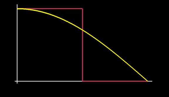
We can view Listing 1 as a digital filter operating on our image data; then we can investigate what the filter does to all the sine waves that compose our texture map. Figure 1 contains a graph of the frequency response of the pixel-averaging filter; the x-axis represents the frequencies of waves in our input image, and the y-axis shows the magnitude by which they're multiplied to get the output.

To perfectly eliminate aliasing, we want a filter that matches the brown line in Figure 1 -- zero amounts of high frequencies, full amounts of low frequencies. In signal-processing terms, we want an ideal low-pass filter. The graph shows that the pixel-averaging filter doesn't come very close to this. It eliminates a big chunk of the stuff we want to keep, which makes the output blurry; it keeps a lot of stuff we'd rather get rid of, which causes aliasing. This is important: switching to a smaller mipmap for rendering will not eliminate as much aliasing as it could, because we accidentally baked some aliasing into the smaller texture.

Figure 1: Frequency response of the box filter versus the ideal. Brown: ideal frequency response, yellow: box filter. The x axis represents frequency; the y axis represents the amount by which the filter scales that frequency (a value between 0 and 1).

How to Build a Better Filter

It's well-established what we must do to achieve an ideal low-pass on our input texture. We need to use a filter consisting of the sinc function, where sinc(x) = sin(πx)/ πx, with x indicating the offset of each pixel from the center of the filter. (At the center, x = 0; recall the Fun Calculus Fact that lim x->0 sin(x)/x = 1.) The problem with sinc is that it's infinitely wide; you can go as far as you'd like along positive or negative x, and sinc will just keep bobbing up and down, with an amplitude that decreases slowly as you zoom toward infinity. Filtering a texture map with sinc would require an infinite amount of CPU time, which is a bummer.

We can compromise. First we decide how much CPU we want to spend building mipmaps; this roughly determines the width of the filter we can use. Then we construct an approximation to sinc, up to that width, and use the approximation to filter our images. We could create our approximation by just chopping off the sinc function once it reaches our maximum width, but this introduces a discontinuity that does bad things to the output. Instead, we multiply sinc by a windowing function; the job of the windowing function is to ease the sinc pulse down to zero, so that when we chop off the ends, badness is minimized.

For a very accessible description of why sinc is the appropriate filter, and how windowing functions work, see the book "Jim Blinn's Corner: Dirty Pixels" (in the References).

So, to design our mipmap creation filter, we just need to choose a filter width (in texture map pixels) and a windowing function. Windowing functions tend to look similar when you graph them, but the differences matter. Filters are funny that way: they're just arrays of real numbers, but just small tweaks to those numbers can significantly change the output. (If you start with a good filter and tweak the coefficients arbitrarily, know that the result is most probably bad.)

Each windowing function represents a different compromise between blurring and aliasing. We can predict what the window will do by graphing the frequency response of the resulting filter, as we did in Figure 1; or we can write some experimentation code that builds mipmaps with arbitrary filters, and look at the results. This month's sample code does just that.

Filters We've Tried

We tried out several filters. The first is the point filter, which is what you get when you just pick one value from every 4 pixels and use that in the lower-level mipmap. (For textures displayed at a scale of 1 texture pixel per screen pixel, it's also equivalent to rendering without mipmapping.)

The second filter is pixel-averaging, the algorithm given in Listing 1.

Third, we gave the Lanczos-windowed sinc function a try, since Jim Blinn says good things about it in his book, and it is popular among graphics programmers.

Fourthly, we look at the Kaiser window. Don Mitchell recently did some experiments revealing that the Kaiser window, with alpha parameter 4, is noticably better than Lanczos for graphics purposes. Don's been around enough to have a filter named after him, so it seemed prudent to pursue this.

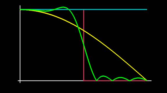
Figure 2 shows the frequency responses of all these filters. The coefficients for the Kaiser filter are only subtly different from the Lanczos filter, so their frequency responses are almost the same. Eyeing images on the screen that were mipmapped by each, I can't see the difference. Mipmapping is not a very strenuous application of image filtering, though; Don's tests were more hardcore. I figure that, so long as the computational expense is the same, we should be in the habit of using the slightly better filter, so it's all warmed up for more difficult future problems.

Listing 1: A common method of building mipmaps, known as "pixel-averaging" or "box-filtering".

void build_lame_mipmap(Mipmap *source, Mipmap *dest) {

assert(dest->width == source->width / 2);

assert(dest->height == source->height / 2);

int i, j;

for (j = 0; j < dest->height; j++) {

for (i = 0; i < dest->width; i++) {

int dest_red, dest_green, dest_blue;

// Average the colors of 4 adjacent pixels in the source texture.

dest_red = (source->red[i*2][j*2] + source->red[i*2][j*2+1]

+ source->red[i*2+1][j*2] + source->red[i*2+1][j*2+1]) / 4;

dest_green = (source->green[i*2][j*2] + source->green[i*2][j*2+1]

+ source->green[i*2+1][j*2] + source->green[i*2+1][j*2+1]) / 4;

dest_blue = (source->blue[i*2][j*2] + source->blue[i*2][j*2+1]

+ source->blue[i*2+1][j*2] + source->blue[i*2+1][j*2+1]) / 4;

// Store those colors in the destination texture.

dest->red[i][j] = dest_red;

dest->green[i][j] = dest_green;

dest->blue[i][j] = dest_blue;

}

Avoiding Ripples

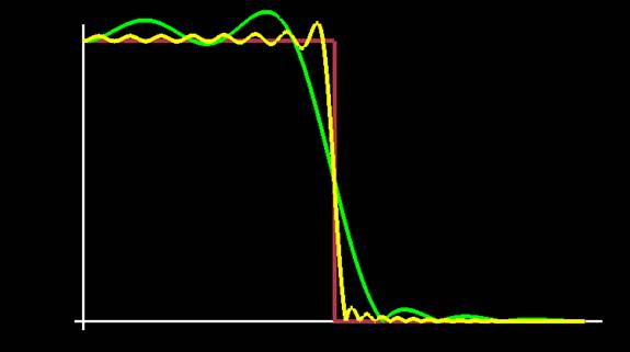
You can see from Figure 2 that there are some ripples in the frequency responses of the higher-quality filters. Signal processing math says that we can increase the quality of these filters just by making them wider. When we do this, we get a curve that more closely approximates the ideal low-pass filter; but it has more ripples, and each peak and trough is concentrated on a tighter group of frequencies. Figure 3 contains a graph of the Kaiser filters for sizes of 16 and 64 samples.

In the world of audio processing, it's common to ignore ripple of this magnitude, but our eyes are pickier than our ears. As those ripples become concentrated around tighter (more coherent) frequency groups, they create more coherent visual artifacts in the image. Pick a wide enough filter, apply it to a texture map that has large areas of constant color, and you've got artifacts ("ringing") all over the place.

I was only able to crank the width of the Kaiser filter up to 14 samples before I started seeing prominent ringing in some test images. To show what happens beyond that, I ran a wide filter on the texture of a road sign. Figure 4 compares the ringing induced for filters at widths of 14 and 64 samples.

One might think that, if you were willing to spend a lot of CPU time, you could use a filter so huge, that is so close to approximating the ideal low-pass response, that you wouldn't see the ripples. I tried this for filters up to 1000 samples wide, and the amount of ringing never seems to decrease.


Figure 2: The frequency responses of filters discussed in this article. Brown: ideal, cyan: point filter, yellow: box filter, green: Lanczos- and Kaiser-windowed sinc pulses (the graphs coincide very closely). The x axis represents frequency; the y axis represents the amount by which the filter scales that frequency.	Figure 3: Frequency responses of Kaiser filters at different filter widths. Brown: ideal, green: 16 samples, yellow: 64 samples. The x axis represents frequency; the y axis represents the amount by which the filter scales that frequency.


Figure 4a: Ringing induced by a 16-sample Kaiser filter.	Figure 4b: Ringing induced by a 64-sample Kaiser filter.

Preventing the Propagation of Distortion

So we're restricted to relatively narrow filters; their frequency responses will be better than the box filter, but there will be some distortion that we can't avoid. Fortunately, we can reduce that distortion's influence on our images.

When we sit down to create a mipmap generator, we often think up the following procedure: take an input image of some width, perhaps 256, and pump it through a mipmapping function that returns a texture 128 pixels wide. Then take that result, push it through the same function, and get back a texture 64 pixels wide. Repeat until it's gotten as small as you need.

This technique causes problems because the output of each filtering step, which contains distortion due to the imperfect filter, is used as input to the next stage. Thus the second stage gets doubly distorted, the third stage triply distorted, etc.

We can fix this by starting fresh from the top-detail image when generating each mipmap level. We still want an ideal low-pass filter, but we want to vary the filter's cutoff frequency. (For the first mipmap level, we want to throw out 1/2 of the frequencies; for the second, we want to discard 3/4; for the third level, 7/8, etc.) To accomplish this, we progressively double the width of our filter and tweak the parameters so the sinc pulse and the window become wider too. (It is okay to make the filter wider, and introduce more ripples, because the size ratio between the source and destination images gets larger). This procedure provided the highest-quality results.

The Sample Code

This month's sample code demonstrates these filters acting on a bunch of sample images. The code is built for versatility and understanding, not speed; it's meant to serve as a code base for you to experiment with. It uses only simple OpenGL calls, so it should work for most people; it's been tested on a few GeForce and Radeon cards. But given the deplorable state of PC hardware these days, I feel lucky if I can even boot up a machine that has a graphics card plugged into it.

By running the sample code, you can browse through textures and see the results of each filter on them. To emphasize the difference between box filtering and Kaiser filtering, there's also a "fillscreen mode" that you can toggle by pressing "f". This tiles the entire screen with the current mipmap; pressing the spacebar switches filters. You can see the effect of the whole screen getting slightly sharper.

The Results

In general, the output images from the Kaiser filter look better. Some examples:

Figure 5 shows a billboard from Remedy Entertainment's Max Payne. In the pixel-averaged version, three mipmap levels down, the copyright notice along the bottom of the billboard has disappeared, and the woman's mouth is something of a blur. In the Kaiser-filtered version, the copyright notice is still visible and the woman's teeth are still easily distinguishable.

Figure 6 shows another billboard. In the box-filtered version, the text is more smudged and indistinct, and the bottle label is less clean-cut.

From the sample app you can also see that once the images get small enough, the choice of filter doesn't matter much; you just get a mess of pixels either way.


Figure 5a: A texture from Max Payne.	Figure 5b: Results of box-filtered mipmapping, zoomed in on the lower-right corner of 5a. Enlarged with Photoshop's bicubic filter.	Figure 5c: Results of Kaiser-filtered mipmapping, zoomed in on the lower-right corner of 5a. Enlarged with Photoshop's bicubic filter.


Figure 6a: Another texture from Max Payne.	Figure 6b: Results of box-filtered mipmapping, zoomed on the upper-right corner of 6a. Enlarged with Photoshop's bicubic filter.	Figure 6c: Results of Kaiser-filtered mipmapping, zoomed on the upper-right corner of 6a. Enlarged with Photoshop's bicubic filter.

Next Month

There are some mipmapping quality issues that don't actually have to do with filter choice; we'll confront those, and we'll see if there's anything we can do to eliminate this problem of wide filters causing our output images to ring. We'll aso question the appropriateness of the Fourier Transform.

Acknowledgements

We thank Remedy Entertainment for allowing us to use images from Max Payne for this article and the accompanying sample code.

The "Phoenix 1 Mile" texture is by Dethtex [original URL no longer valid].

Thanks to Don Mitchell, Sean Barrett, Chris Hecker, and Jay Stelly for fruitful discussion.

References

Alan Watt and Mark Watt, Advanced Animation and Rendering Techniques: Theory and Practice, Addison-Wesley. Chapter 4 talks about anti-aliasing and how mipmapping approaches the problem.

Jim Blinn, Jim Blinn's Corner: Dirty Pixels, Morgan Kaufmann Publishers. Chapter 2 talks about aliasing, and chapter 3 uses the Lanczos window for image filtering.

R.W. Hamming, Digital Filters, Dover Publications. Talks about why, from a fundamental standpoint, it's a good idea to look at sampled sequences as being built out of sine waves.

Ken Steiglitz, A Digital Signal Processing Primer, Addison-Wesley. A very readable, down-to-earth discussion of how filters work and how to make them. Recommended for those who find most DSP books too stifling or impenetrable.