The Inner Product, July 2003
Jonathan Blow (jon@number-none.com)
Last updated 16 January 2004
 

Unified Rendering Level-of-Detail, Part 5 (The Last!)

Related articles:

Rendering Level-of-Detail Forecast (August 2002)
Unified Rendering LOD, Part 1 (March 2003)
Unified Rendering LOD, Part 2 (April 2003)
Unified Rendering LOD, Part 3 (May 2003)
Unified Rendering LOD, Part 4 (June 2003)

Note: This article is currently missing Figure 2. 
We will attempt to remedy this situation in the future.

This series of articles is about LOD for large triangle soup environments. Such environments must be divided into chunks; the biggest issue in this kind of system is filling in the holes between neighboring chunks at different levels of detail. I fill these holes with small precomputed triangle lists called "seams", and earlier in this series I showed how to construct those seams.

In part 3 we saw how to split a single chunk of geometry into two, and how to generate the initial seam between them. Last month, in part 4, we saw how to split a chunk that is connected via a seam to another chunk, while maintaining existing manifolds. I mentioned that this is sufficient to build a chunked BSP tree of the input geometry; I showed some code that split the Stanford Bunny by arbitrary planes and played with the LOD of the various pieces.

This month I'll begin with that basic premise of building a chunked BSP tree; before long we'll be rendering a large environment with this system (and not just a bunny).

We'll focus on three major parts of the algorithm: (1) dividing the environment into initial chunks, (2) putting those chunks together into a detail-reduced hierarchy, (3) choosing which levels of the hierarchy to display at runtime.


(1) Dividing the environment

We don't want to assume anything about the shape of the environment. Maybe it's a big localized block like an office building, or maybe it's a loose set of tunnels that curve crazily through all three dimensions. An axis-aligned approach to segmenting the geometry, like a grid or octree, would work well for the office building but not for the tunnel. The chunked BSP treatment is nice because it doesn't much care how pieces of the environment are oriented.

I needed a method of computing BSP splitting planes. Most game-related BSP algorithms divide meshes at a 1-polygon granularity, so to acquire a splitting plane they pick a polygon from the mesh and compute its plane equation. But that's the kind of thing I am trying to get away from -- thinking too much about single triangles is a violation of the spirit of the algorithm. I want a more bulk-oriented approach, so I statistically compute a plane that divides the input into two sub-chunks of approximately equal triangle counts.

There are other things I might wish to do, besides just minimize the difference in triangle count between the two sub-chunks. I might wish to produce sub-chunks that are as round as possible, so that we don't end up with a scene full of long sliver-chunks. I might wish to balance the number of materials used in each chunk. Most probably, I'd whip up a heuristic that combines many parameters and makes trade-offs to achieve a happy medium.

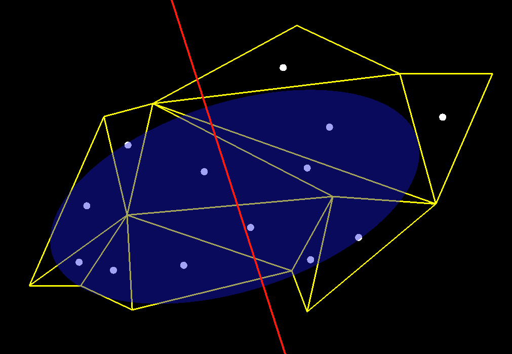
To compute the splitting plane in a quick and dirty way, I treat the chunk as a bunch of point masses, one mass located at the barycenter of each triangle. I then compute the vector-valued mean and variance of these masses (see "My Friend, the Covariance Body", Game Developer magazine, September 2002). This gives me an ellipsoid that summarizes the mass of the chunk, as though that mass were normally distributed. I then split that ellipsoid in half, using a splitting plane that passes through its center and spans the ellipsoid's two minor axes. I use the minor axes because this produces halves of minimum eccentricity -- in other words, pieces that are "the most round". (We might produce pieces that are more nicely-shaped by choosing not to split the ellipsoid through the center). See Figure 1 for a 2D illustration of the splitting-plane computation.
 

Figure 1: Some triangles (yellow); their barycenters (white dots); the ellipsoid, drawn at 1.7 standard deviations, that we get from treating these barycenters as point masses (blue); and a splitting plane that spans the minor axes and passes through the center of the ellipsoid (red).

(2) Combining chunks into a hierarchy

Our LOD rendering algorithm doesn't place many constraints on the way we organize our chunks. It just wants an n-ary tree with hierarchical bounding volumes that help us choose detail levels. We'll talk about computing those volumes in part (3); for now we'll just discuss putting the chunks together.

First, we need to decide on a policy about which chunks to combine. The easiest choice is just to use the hierarchy that was created by the BSP splits. We combine two chunks into one, detail-reducing to a given triangle budget at each level, until we once again reach the root of the BSP tree.

This is easy because we don't have to think much, and in fact it's the first thing I implemented. Clearly, though, it may not produce the best results. For one thing, in any tree structure like this we end up with nodes that are neighbors spatially, but that are far apart in the hierarchy. In terms of scene quality it may be best to combine these nodes early, but they won't be combined until the level of detail becomes very low. Secondly, we probably want the freedom to combine more than two chunks at once. The pre-ordained BSP hierarchy does not give us much freedom.

So instead, I just take the chunk geometry stored on the leaves of the BSP tree, throwing away the tree structure itself. Then I cluster the chunks using a heuristic that is independent of the original chunking process. This lets me match any number of chunks together, building a new n-ary tree from the leaves to the root. At each level of the n-ary tree, I combine the participating chunks and seams into one mesh, and then run a static LOD routine on that mesh. This is the same thing I did with the terrain hierarchy from Parts 1 and 2, but now the environment representation is less restricted.

You can imagine many different policies for choosing the triangle budget for each node in this geometric hierarchy. In the sample code, my heuristic is that each node should have approximately the same number of triangles (for example, 4000). So the BSP splits occur until each leaf has about 4000 triangles; then I discard the BSP tree and begin combining leaves 4 at a time, LOD'ing each combination back down to 4000 triangles. So in the end, I have a 4000-triangle mesh at the root that represents the entire world, with subtrees containing higher-resolution data.


(3) Choosing which resolution to display at runtime

So we've got these hierarchical chunks representing world geometry; at runtime we need to choose which chunks to display. Typically, LOD systems estimate the amount of world-space error that would be incurred by using a particular level of detail; they project this error onto the screen to estimate how many pixels large it is, then use that size-in-pixels to accept or reject the approximation.

Algorithms from the Continuous LOD (CLOD) family tend to perform this operation for each triangle in the rendered scene. We want to operate at a larger granularity than that. We could do that as follows: for each chunk, find the longest distance by which the LOD'd surface displaces from the original, pretend this error happens at the point in the chunk that is nearest to the camera, and use the corresponding z-distance to compute the error in pixels.

It's customary in graphics research to take an approach like this, since it's conservative: you can achieve a quality guarantee, for example, that no part of the chosen approximation is rendered more than 1 pixel away from its ideal screen position.

But with graphics LOD, this kind of conservativism is not as fruitful as one might assume. When choosing LODs based on the distance by which geometry pops, we ignore warping of texture parameterizations, changes in tangent frame direction, and transitions between shaders. The popping distance can be vaguely related to some of these things, but in general it only controls a portion of the rendering artifacts caused by LOD transition. Even with a strict bound on popping distance, we're not achieving a guarantee about the quality of the rendered result.

In addition, this conservative approach can be harmful to performance. To provide that somewhat illusory guarantee, the algorithm must behave quite pessimistically (for example, assuming that the maximum popping error occurs at the position in the chunk closest to the camera at an angle that is maximally visible). This causes the algorithm to transition LODs earlier than it should need to.

I suggest we acknowledge the fact that, when tuning LOD in games, we just tweak some quality parameters until we find a sweet spot that gives us a good balance between running speed and visual quality. So it doesn't matter how many pixels of error a particular LOD parameter represents, because we don't set the parameter by saying "I want no more than 0.7 pixels of error", we set it by tweaking the pixel-error threshold until we decide that the result looks good -- whatever number of pixels is produced by that tweaking, that's what the answer is. Conservative bounds are not specially meaningful in this situation.

In this month's sample code, I approximate the spatial error for a given LOD without using a conservative worst case. I do this by finding the root-mean-square of all the spatial errors incurred during detail reduction. Recall that I'm using error quadric simplification, so squared spatial errors are easy to query for. I just take each quadric Q and zero out the dimensions having to do with texture coordinates, which gives me Q'. Then I find v^TQ'v where v is the XYZ-position of a vertex in the reduced mesh and Q is its error quadric. That product yields the squared error; I find the mean of all those errors and square-root that mean.

This gives me an error distance in world-space units. I use this distance to compute a bounding sphere centered on the chunk, whose radius is proportional to the error distance. If the viewpoint is outside the sphere, we are far enough from the chunk that we don't need more detail, so we draw the chunk. If the viewpoint is inside the sphere, we need more detail, so we descend to that chunk's children.

The radius is proportional to the error distance because perspective involves dividing by view-space z. For chunks within the field of view, view-space z is approximately equal to the world-space distance from the camera to the chunk, which is why world-space bounding spheres make sense. The constant of proportionality is the LOD quality level, which you can adjust at will. You just need to make sure that the spheres are fully nested in the chunk hierarchy, which means potentially expanding each node's sphere to enclose its childrens' spheres.

These spheres can be viewed as isosurfaces of continuous-LOD-style pixel error projection functions. For more in the way of explanation, see my slides from Siggraph 2000, as well as Peter Lindstrom's paper (For More Information). Both references describe Continuous LOD schemes, so I don't recommend you implement either, but the discussion of isosurfaces can be useful.

Trash talk time: Lindstrom disses my CLOD algorithm from 2000 in his paper, but his criticism is misguided. Most of the attributes that he scorns are actually important design decisions, chosen to create an algorithm that behaves reasonably under heavy loads. Not seeing this, he champions features that I intentionally discarded, features that inherently make for a poorly-performing system. (I mean come on, Peter -- given anything like real-time requirements, a persistent orientation-sensitive LOD metric is just a fundamentally bad idea. So why make your algorithm more complicated, and slower, in order to support that capability?)

I shouldn't single out Lindstrom, because this general problem pervades much of academic computer graphics. Be careful when you read those Siggraph papers; the authors don't have the same design priorities that you do. In general these authors don't do proper cost/benefit analyses of their algorithms. The "previous work" section is just about convincing you that the authors have done some homework; it says nothing about whether the authors are honestly considering the relative advantages and drawbacks of their system with the previous work. The performance numbers featured in "results" sections are a sales device; they say little about how an algorithm will really perform, since the authors rarely develop their systems for real-world data sets.

Okay, enough trash talk. Back to talking about nested spheres. To keep things simple, I have so far pretended that we perform an LOD transition exactly when the viewpoint crosses one of those spheres. But as you know from Part 2, we actually want to fade slowly between LODs. In the sample code this is done by computing two radii, one which is greater than the instant-transition radius, and one which is less than it. LOD fading begins when the viewpoint crosses one sphere, and ends when it crosses the other.

You can easily imagine more sophisticated methods of computing LOD sphere radii. Perhaps we want to render approximately the same number of triangles every frame, no matter where the player is standing in the environment. We could run an energy minimization system at preprocess time, expanding and contracting the spheres until we achieve something close to the desired result. Or instead of tweaking radii, we could leave radii fixed and adjust the actual number of triangles used in each LOD chunk.


Sample Code and Future Work:

This month's sample code preprocesses and renders Quake 3 .bsp files. You can see the results for one such environment in Figure 2.

The code is not yet a plug-and-play tool for general use. However, I plan to keep working on this system in the future. Even though this is the last article about this algorithm (for now?), I will post new versions of the code on the web as improvements occur. If you have any input on how to make this LOD system maximally useful, let me know!

Because we're storing triangle soup meshes, the file size for the environment might be very large. It takes a lot more space to store a mesh of a heightfield terrain than it does just to store the height samples! To alleviate this problem, we may wish to investigate mesh compression. Perhaps that will be a good topic for some future articles....


References

J. Blow, "Terrain Rendering Research for Games", slides from Siggraph 2000. Available at http://www.red3d.com/siggraph/2000/course39/S2000Course39SlidesBlow.pdf

P. Lindstrom and V. Pascucci, "Visualization of Large Terrains Made Easy", Proceedings of IEEE Visualization 2001. Available at http://www.cc.gatech.edu/gvu/people/peter.lindstrom/

S. Gottschalk, M. C. Lin and D. Manocha, "OBB-Tree: A Hierarchical Sturcture for Rapid Interference Detection", Siggraph 1996. Available at http://citeseer.nj.nec.com/gottschalk96obbtree.html
 

Figure 2 (missing currently!)

2a: Quake 3 level "hal9000_b_ta.bsp", by John "Hal9000" Schuch, rendered using the LOD system. 2b: Level chunks have been artificially moved away from each other so you can see the seams (red bands). 2c: Chunks have been drawn with color-coding that shows their resolution level.